Learning the Exit (part 1)
I have a model that indicates mean reversion with ~81% accuracy. Here is an example of a MR scenario the model identified:
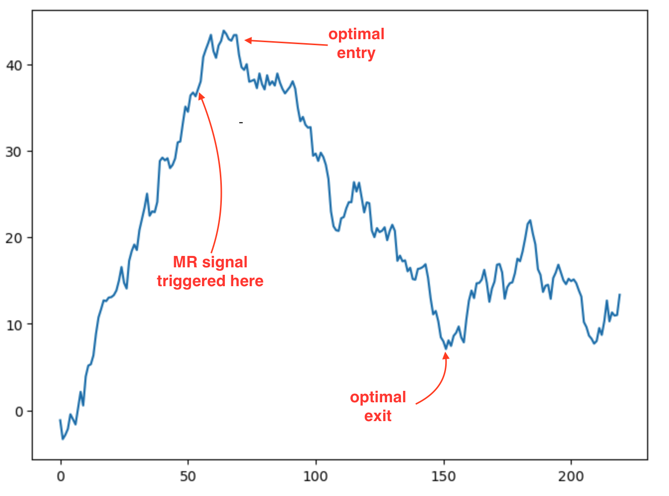
The strategy is very good at detecting entry points (usually very close to optimal), however is fairly crude in terms of how it determines the exit. Given that 81% of MR (with this model) experiences a profit of at least 25% of the prior amplitude, one could take the approach of waiting for a pullback of 25% less stop-loss.
While there are various profitable fixed stop-loss and profit target regimes for this model, using a fixed target ignores market information post entry. Here are some problems I want to solve:
- opportunity cost
- The average profit available is ~150% of the prior amplitude (due to the scenario this model detects).
- Selecting a conservative fixed exit target leaves “money on the table”
- risk reduction
- many of the risky scenarios involve a runaway trend post signal; this is detectable
- blindly holding for a k% exit, ignoring information post entry, does not make sense
Approaches
We might start with a labeling approach using the Labeler to identity the target mean-reversion extent. The labels would indicate whether we should enter, build position, reduce, or exit. Given the labels, we can attempt to construct a ML driven model :
- supervised classifier to predict individual labels (not recommended)
- This is unlikely to work without significant noise or lag. The features may not have support for all movements or periods in the movement. For example some movements may be associated with significant directional volume and others might not be. Forcing a model to be able to predict all points in the timeseries is doomed to failure.
- learn a policy
- Using either RL (Reinforcement Learning) or GP (Genetic Programming), learn a policy to decide what action to take at any point in time. These algorithms are not (may not) be penalized for missing opportunities, rather can focus on learning detectable scenarios.
- we can make use of the labeler to inform the policy we are trying to learn; However, unlike classification, we are not “forcing” the model to learn every label. More on this when we discuss the reward function in the next post.
I will focus on learning a policy in this post.
Application of RL
There are many great papers and tutorials for reinforcement learning, so will not go into great detail here. Our goal is to create a model that decides how to trade our MR exit. RL is framed as a markov process, where we progress from one state \(s_t\) to the next \(s_{t+1}\), based on the action \(a_t\) taken by a “policy function” \(\pi_{\theta}(a | s_t)\).
Given our entry signal, the policy function \(\pi_{\theta}(a | s_t)\) will propose an action \(a_t\) for each bar post MR signal, informing how to trade the prospective MR entry and exit. The actions it takes can either be discrete (for example Buy, Sell, None) or continuous (such as % allocation) in nature.
We learn \(\pi_{\theta}(a | s_t)\) by training the policy function across many “episodes”. In our case an episode starts with the MR signal at time \(T_{start}\) and ends within some maximum holding period \(T_{start} + \Delta T\). Reinforcement learning requires some form of feedback in order to effect learning, this is accomplished by assigning a reward \(r(a_t,s_t)\) for each action given a state. The learning process attempts to learn a policy function that maximizes the accumulated reward across episodes (roughly speaking).
For a given episode, there will be an optimal sequence of actions \(a_{t = 0} .. a_{t=T}\) that maximizes the cumulative reward function \(Q(s_t,a_t)\). In Q learning, this cumulative reward function is expressed as (source wikipedia):
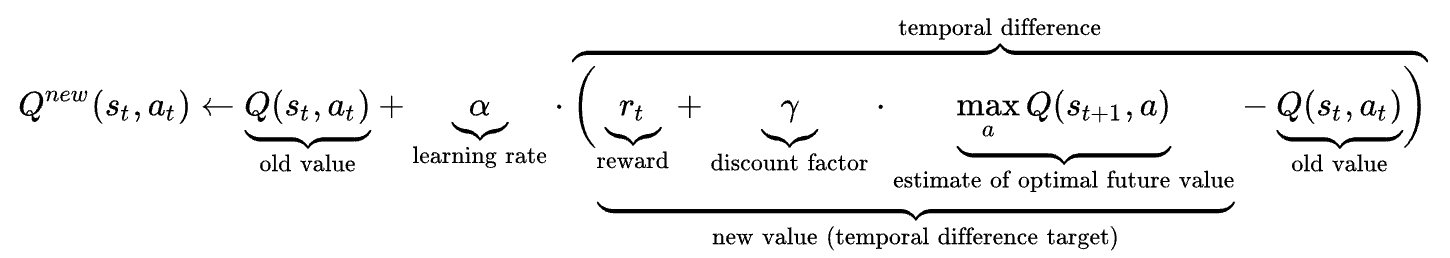
Note that the above expression is only applicable to discrete action spaces. Q-learning was an early implementation of reinforcement learning, later superseded by a variety of more effective deep-learning based approaches, such as:
- A2C
- DQN
- DDPG
- …
Example
For example in the entry and exit scenario pictured here:
the optimal action sequence for an episode in our MR trading might be:
{ \(a_0\) = None, .., \(a_9\) = None, \(a_{10}\) = Sell, \(a_{11}\) = None, …, \(a_{80}\) = Buy }
In the above example:
- the (downward) MR signal was early by 10 bars (the market continued to climb for 10 bars); hence the optimal action would be “no action” in the first ten bars.
- the agent entered short at bar 10 and exited at bar 80.
Entering earlier would have reduced the cumulative reward, as an earlier entry would have resulted in negative reward for \(a_0\) through \(a_10\). Likewise, entering later, say at \(a_20\), would have reduced the cumulative reward due to opportunity cost, not having harvested the rewards from \(a_10\) to \(a_20\).
Sub-Problems
Breaking this down into sub-problems:
- determine feature set & state likely to support policy learning
- in addition to features want state indicating current position, P&L within episode, etc.
- defining a “gym” where the agent trains on episodes (collection of MR entries and timeseries post prospective entry)
- track current state given actions and environment
- compute reward
- determine reward approach
- what is the best way to reward so that our training converges towards a model with desireable behavior?
- determine actions
- discrete or continuous action spaces: for example Buy, Sell, Hold (discrete) versus % allocation (continuous).
I will focus on the reward function in the next post.