Feature Selection (3 / 3)
Random Forest vs Information Geometric Approach
In the prior two posts, investigated:
- Subspace Projections: feature selection (1/3)
- Information Geometric: feature selection (2/3)
In this post will evaluate feature importance as implemented by Random Forest and compare to Information Geometric approaches. Here is an outline of what would like to discuss:
- similarities between Decision Trees and Information Geometric approaches for feature selection
- some of the deficiencies of Decision Trees
- some areas for improvements
As we will see, Random Forest’s approach to generating decision trees has some similarities to the information geometric approach.
Algorithm
A random forest is a bagging ensemble method, aggregating 100s or 1000s of decision tree models to determine a classification or regression model. Random Forest will apply the following process:
- generate K trees, for each tree to be generated:
- sample a random subset from the training <feature, label> set
- randomly select a subset of features to be applied in the current tree
- create a decision tree using one of 3 or 4 possible algorithms and splitting criteria
- possibly trim tree to a maximum-depth or adjust tree according to other criteria
- prediction:
- evaluate feature set against each decision tree: each tree will vote with a label
- aggregate votes from each tree using a voting metric -> this determines predicted label
There are many variations of the above.
To understand random forests (and how they can be used for feature selection), lets consider the structure and construction process of a decision tree. Rather than describing the process in detail here would recommend reading How does a Decision Tree decide where to split?, which describe tree structure and splitting decision making.
The decision trees used in random forests are generally binary, and for continuous variables, split on an intercept that, using a probability metric, tries to weigh classes evenly so that the left and right children are predominantly class 0 and class 1 respectively (for a binary classifier).
Example
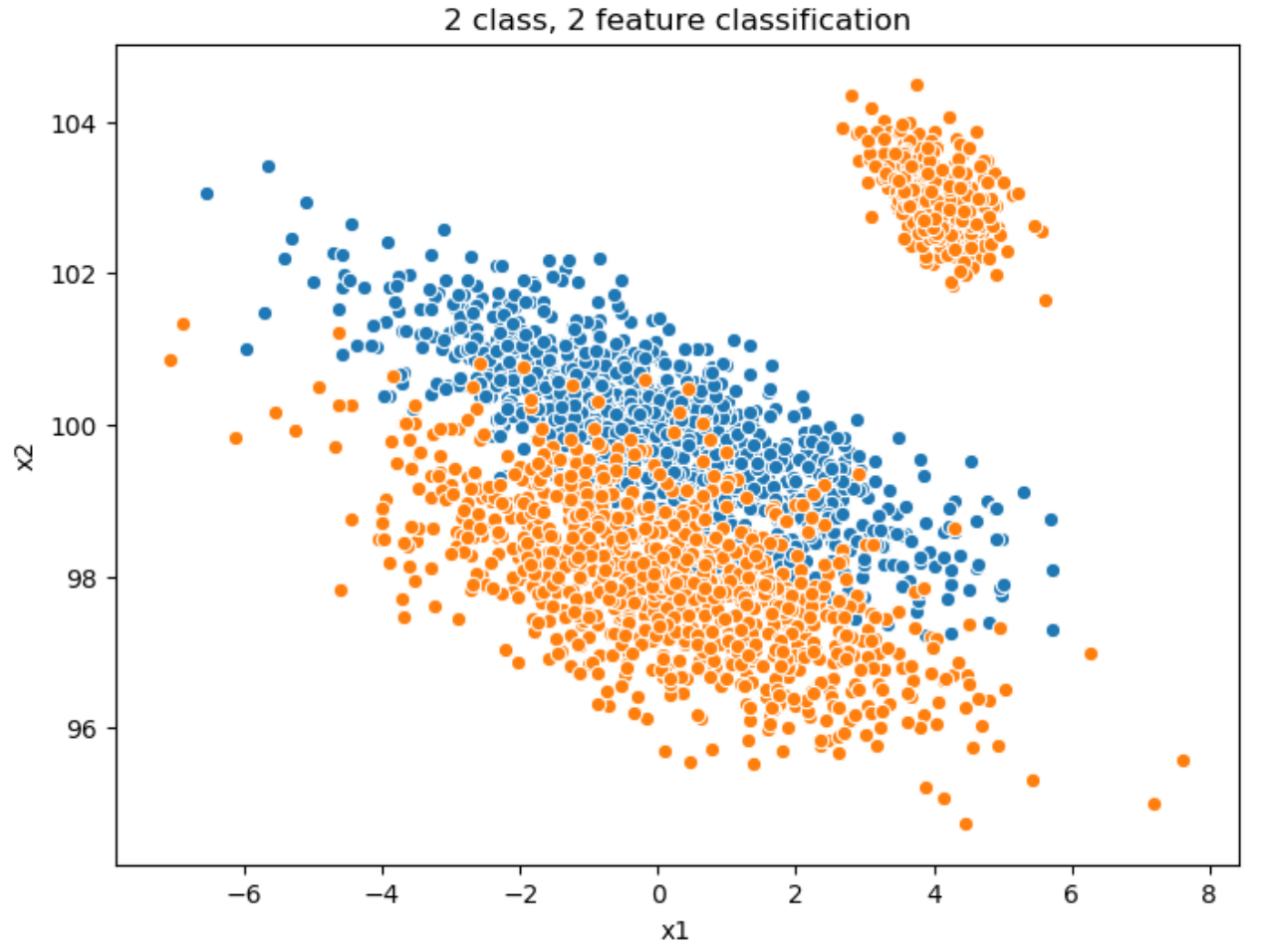
Let’s create a 2-dimensional feature set for a binary classification problem. I will use this to discuss tree construction, information geometry, and feature selection:
(see appendix for full code)
label0 = rand2d (n = 1000, mu = [0, 100], sigmas=[2.0, 1.0], corr = -0.8)
label0["label"] = 0

label1 = pd.concat([
    rand2d (n = 1000, mu = [0, 98], sigmas=[2.0, 1.0], corr = -0.6),
    rand2d (n = 300, mu = [4, 103], sigmas=[0.5, 0.5], corr = -0.5)
])
label1["label"] = 1

all = pd.concat([label0, label0])

sns.scatterplot (label0.x1, label0.x2),
sns.scatterplot (label1.x1, label1.x2).set_title("2 class, 2 feature classification")
Steps
The decision tree is built, as a binary tree, from the root downwards. The algorithm does the following at each step:
- decide which feature offers the most discrimination given the residual labels at the current node
- based on gini score (you can read up on this in the link provide above), one of the features will be selected for a split
- determine where to effect the split
- this will be of the form: “if x2 < 99”
- 2 child nodes are added to the current node, one for class 0 and the other for class 1
- the left node will contain all (residual) samples where x2 >= 99 (class 0)
- the right node will contain all (residual) samples where x2 < 99 (class 1)
Here is an example of a (partial) decision tree that might be created for the above data:
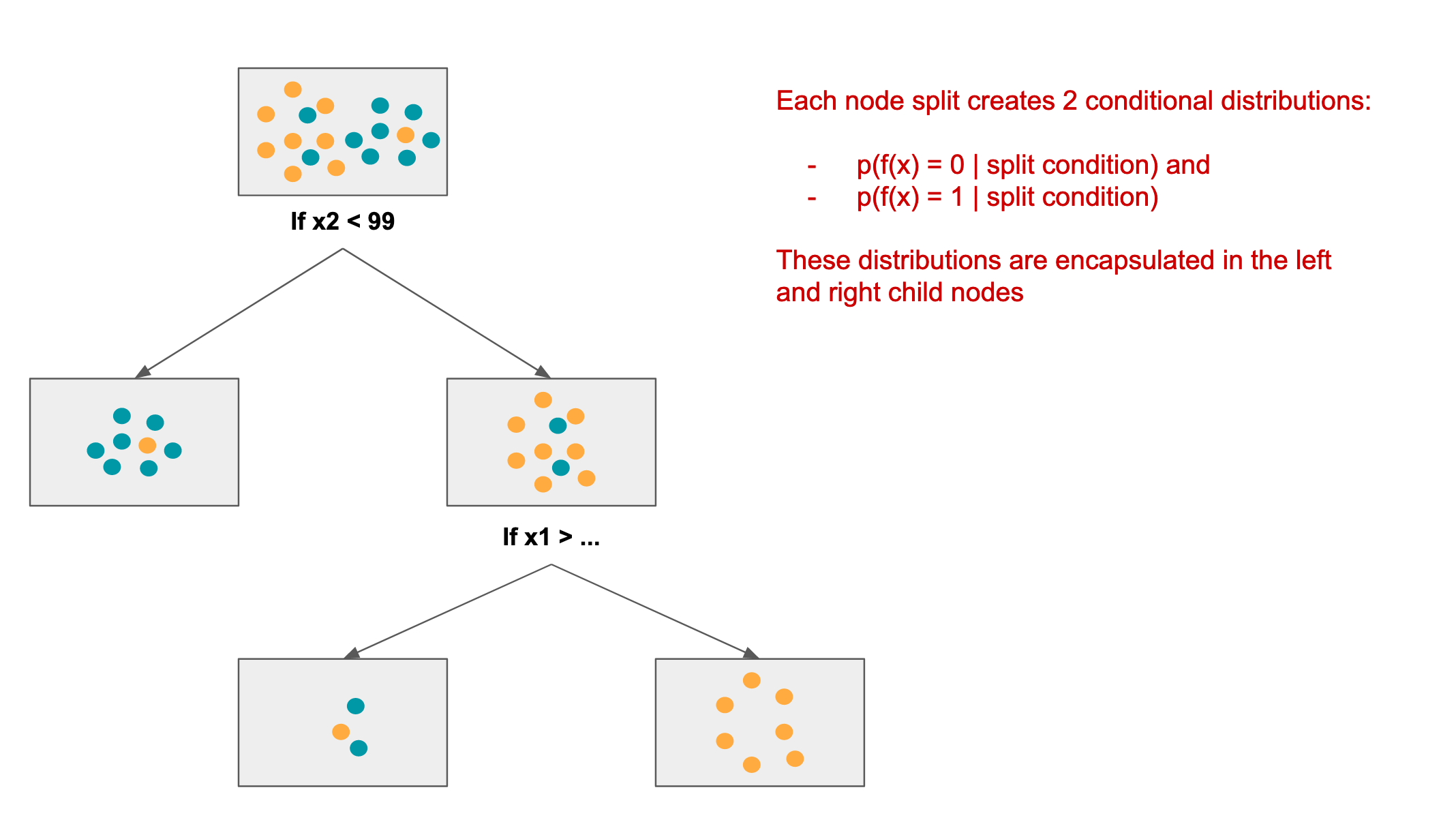
Decision tree node split & relationship to information geometry
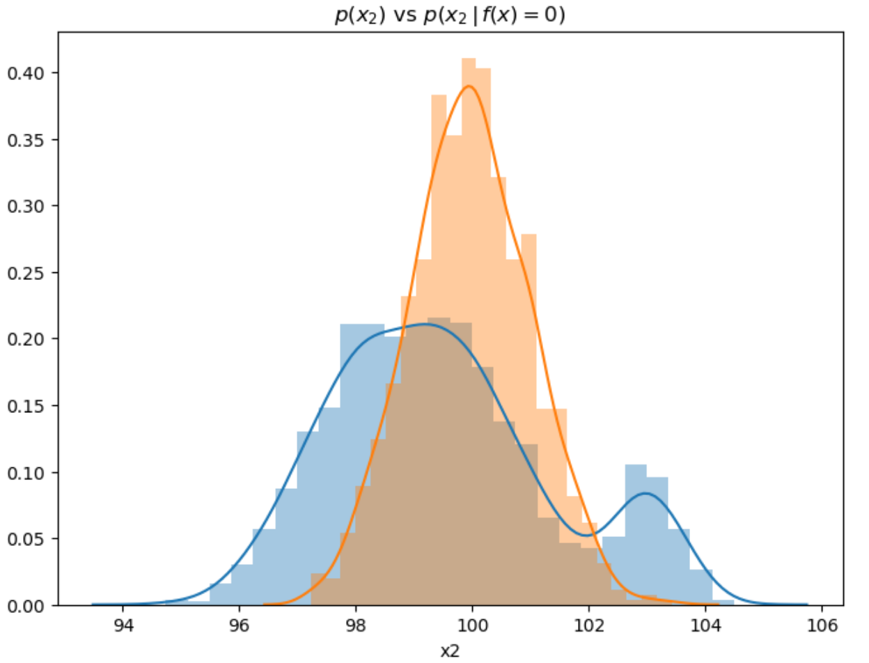
Each split in the decision tree creates an “updated” conditional distribution for each class (in the binary classification case). Gini, Entropy, or Chi-Squared measures are used find a split that maximizes this discrimination. Recall that with our Information Geometric feature selection algorithm, we are also trying to find features that provide the maximum discrimination between classes. For example if we examine the prior and conditional distributions for feature x2 for class = 0:
sns.distplot(all.x2),
sns.distplot(all.x2[all.label == 0]).set_title(r"$p(x_2)$ vs $p(x_2 \, \vert \, f(x) = 0)$")
The distribution (or Information Geometric) approach evaluates the degree of discrimination between prior and conditional distributions with respect to labels. We can see that feature x2 has clear impact on f(x), given that the two distributions are quite distinct.
Let’s look at how random forest tackles class discrimination from a distribution point-of-view. The impact in of the 1st split in the decision tree if x2 < 99:
sns.distplot(all.x2),
sns.distplot(all.x2[all.x2 >= 99]).set_title(r"$p(x_2)$ vs $p(x_2 \, \vert \, x2 \geq 99)$")
The first decision tree split discriminates in a reasonable fashion, however, but needs to trim the right tail and capture some of the mass to the left in the distribution:
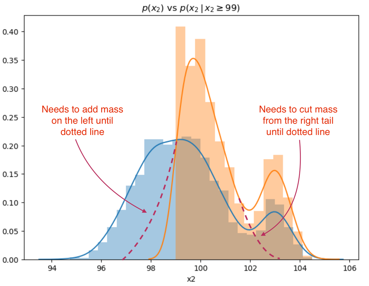
The tree will go on to add and remove “mass” from the conditional distributions at each level and node in the decision tree to the point where either has replicated the sample distribution or has reached stopping criteria.
We can see that there is a similarity between the conditional distributions produced at node splits and conditional distributions based on label. Indeed random forest would endeavor to make the perfect split that would replicate \(p(x_2 \, \vert \, f(x) == 0)\) in one split if it had the latitude to do so.
Issues with Random Forest
Decision trees, by design, only decompose the feature space on orthogonal axes. One could consider more complex partitioning functions, involving 2 or more features per node. For example:
- linear on 2 features (would solve the rotation problem)
- gausian kernel
- …
However the tree-construction complexity might lead to a NP-complete algorithm, and it would be harder to measure and contain model complexity.
Here is a possible set of cuts a decision tree would perform (the first 8 splits) on our sample space in order to properly separate classes:
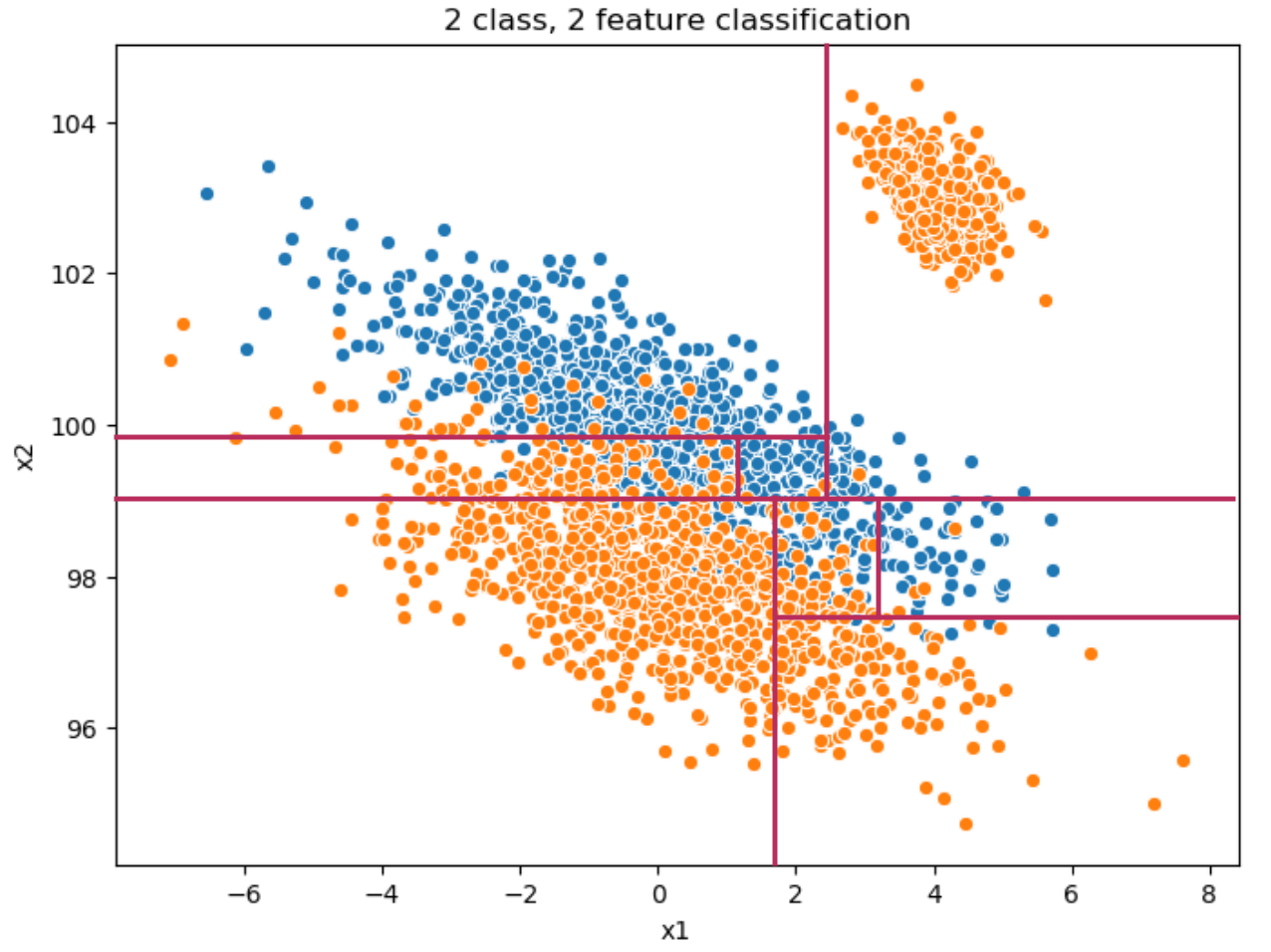
Note that the cuts are always orthogonal to the axis. For class structure with non-orthogonal or rotate alignments (such as the above), a decision tree would need to make many splits to correctly classify up and down the diagonal separating the classes.
While there are other classifiers (for example SVM), which can apply kernels, performing separation in a non-linear space, Random Forest does surprisingly well in spite of its limitations. This is likely due to the non-linearity of averaging all of the different decision trees, allowing for net curvature in separating class regions.
Feature Selection
Feature importance in Random Forest is determined by observing how often a given feature is used and the net impact on discrimination (as measured by Gini impurity or entropy). My approach to determining the best set of features with RF is to:
- evaluate N random folds of the training set, for each data set sample:
- generate a random forest
- extract feature importance as determined by the model (net impact on discrimination)
- aggregate score for each feature
- rank aggregate scores across the N runs and select top-K
Comparison with Information Geometric Approach
It is hard to compare Random Forest and the specific Information Geometric approach I use universally; rather will provide some anecdotes:
- I tend to get a 75% overlap between the top-K random forest features and information geometric approach
- Depending on complexity of distributions (for example are the tails important), the information geometric approach may give better results
- you may want to take the union of the 2 approaches (with a 25% overage on # of features) to retain maximum informational content
Conclusions
Some final thoughts on feature selection:
- is very dependent on composition of data and relationship to features
- for example if f(x) is dependent in a non-linear fashion to the tails in a feature sub-space random-forest may or may not be able to isolate. Information Geometric approach could also fail to recognize importance
- is dependent on target machine learning model
- arguably information in features exists outside of model selected, however, some models may not be able to utilize all of the information in features
- is an imperfect process
It is unlikely to be my last post on feature selection, as am always looking to refine my approach. I will move on to another topic for the next post however.
Appendix: Code
import numpy as np
import seaborn as sns
from scipy.linalg import cholesky
from scipy.stats import norm

def rand2d (n: int, mu = [0, 0], sigmas = [1, 1], corr = 0.0):
    # produce covariance
    v = np.diag(sigmas)
    cor = np.array([[1.0, corr], [corr, 1.0]])
    cov = np.matmul (np.matmul (v, cor), v)

    # get iid random samples
    iid = norm.rvs (size = (2, n))

    # apply covariance
    chol = cholesky (cov, lower = True)
    vectors = np.dot(chol, iid)

    # add mu's
    return pd.DataFrame({'x1': vectors[0] + mu[0], 'x2': vectors[1] + mu[1]})

label0 = rand2d (n = 1000, mu = [0, 100], sigmas=[2.0, 1.0], corr = -0.8)
label0["label"] = 0

label1 = pd.concat([
    rand2d (n = 1000, mu = [0, 98], sigmas=[2.0, 1.0], corr = -0.6),
    rand2d (n = 300, mu = [4, 103], sigmas=[0.5, 0.5], corr = -0.5)
])
label1["label"] = 1

all = pd.concat([label0, label0])

sns.scatterplot (label0.x1, label0.x2),
sns.scatterplot (label1.x1, label1.x2).set_title("2 class, 2 feature classification")

sns.distplot(all.x2),
sns.distplot(all.x2[all.label == 0]).set_title(r"$p(x_2)$ vs $p(x_2 \, \vert \, f(x) = 0)$")

sns.distplot(all.x2),
sns.distplot(all.x2[all.x2 >= 99]).set_title(r"$p(x_2)$ vs $p(x_2 \, \vert \, x2 \geq 99)$")