Feature Selection (2 / 3)
Distribution Based Approaches
As mentioned in the prior discussion feature selection (1/3), of primary interest is understanding the contribution of each feature in \(\vec{x}\) to the outcome or class labeling function \(f(\vec{x})\). One way to examine this is to understand how the distributions:
- \(p(x_f)\), the probability distribution of feature f (without regard to label)
- \(p(x_f\, \vert\, f(x) = y)\), the feature distribution conditional on class label
differ from each other. For a feature with no relationship to the outcome \(p(x_f)\) and \(p(x_f\, \vert\, f(x) = y)\) will not be substantially different distributions. Whereas if \(x_f\) has substantial influence on \(f(\vec{x})\), the conditional distribution \(p(x_f\, \vert\, f(x) = y)\) will be substantially different from \(p(x_f)\).
Illustrative Example
Lets assume that we have 2-dimensional features \(\vec{x} = [ x_0, x_1 ]^T\), where the model we are looking to learn is dependent on the first feature \(x_0\), mapping as \(f(\vec{x}) = \begin{cases} 0 & \text{ if } x_0 < 1.0 \\ 1 & \text{ if } x_0 \ge 1.0 \end{cases}\)
import numpy as np
import seaborn as sns

x0 = np.random.normal (0.0, 1.0, 2000)
x1 = np.random.normal (0.0, 1.5, 2000)
y = (x0 >= 1.0) * 1.0

sns.distplot(x0),
sns.distplot(x0[y == 1]).set_title(r"$p(x_0)$ vs $p(x_0 \, | \, f(x) = 1)$")
Lets compare the distributions \(p(x_0)\) and \(p(x_0\, \vert\, f(x) = 1)\):
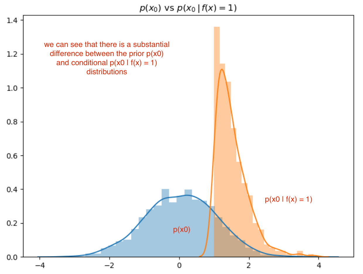
We can clearly see (above) that feature 0 has a strong relationship with the function f(x) given the significant difference between the prior and conditional distributions.
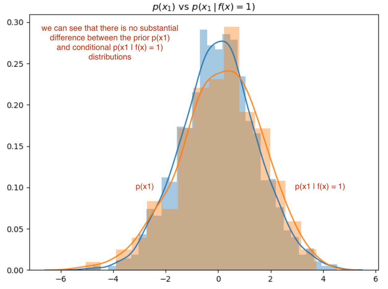
However, in the next figure (below), feature 1 shows no impact on the outcome of f(x); this is evident by the lack of difference between the prior and conditional distributions for feature \(x_1\):
sns.distplot(x1),
sns.distplot(x1[y == 1]).set_title(r"$p(x_1)$ vs $p(x_1 \, | \, f(x) = 1)$")
Implementation Approach
To determine which features have impact on f(x), we can do the following:
- use a distance measure that allows us to compare distributions
- for example Jensen-Shannon, Wasserstein (Earth Mover Distance), …
- normalize distributions into the same space so that distribution distances can be compared
- evaluate CDF of distributions on [0,1] instead of separate native coordinate spaces
- deal with correlation between features
- 2 features with significant impact on f(x) may also be highly correlated
Here are some distance measures we could use in determining the difference between the prior and conditional distributions:
- Jensen-Shannon Divergence
- Formulated along the lines of information entropy, however, where the log probability term is the ratio of probabilities between distributions. This is a symmetric adjustment to Kullback-Leibler Divergence.
- The computational complexity for univariate distributions is O(n) and O(n^k) for multivariate.
- Wasserstein (or EMD)
- A more flexible divergence metric allowing comparison of distributions even when their supports do not intersect
- For the case of univariate empirical distributions has complexity O(n log n) in the number of samples. For multivariate the complexity is O(n^3), though there are some approximate methods linear in time.
At some point will do an analysis to compare how the two perform. For the moment forcusing on Wasserstein distance.
The 1st order Wasserstein distance is known also as the “Earth Mover Distance” (EMD). The approach determines the “amount of work” required to move mass from one distribution to another such that they are equivalent. This amount of work: sum of mass moved over a distance is the EMD metric. In the diagram below we have 2 different distributions with unequal mass / position of mass. The EMD algorithm determines the minimal flow (distance x mass) required to be moved to equalize the distributions:
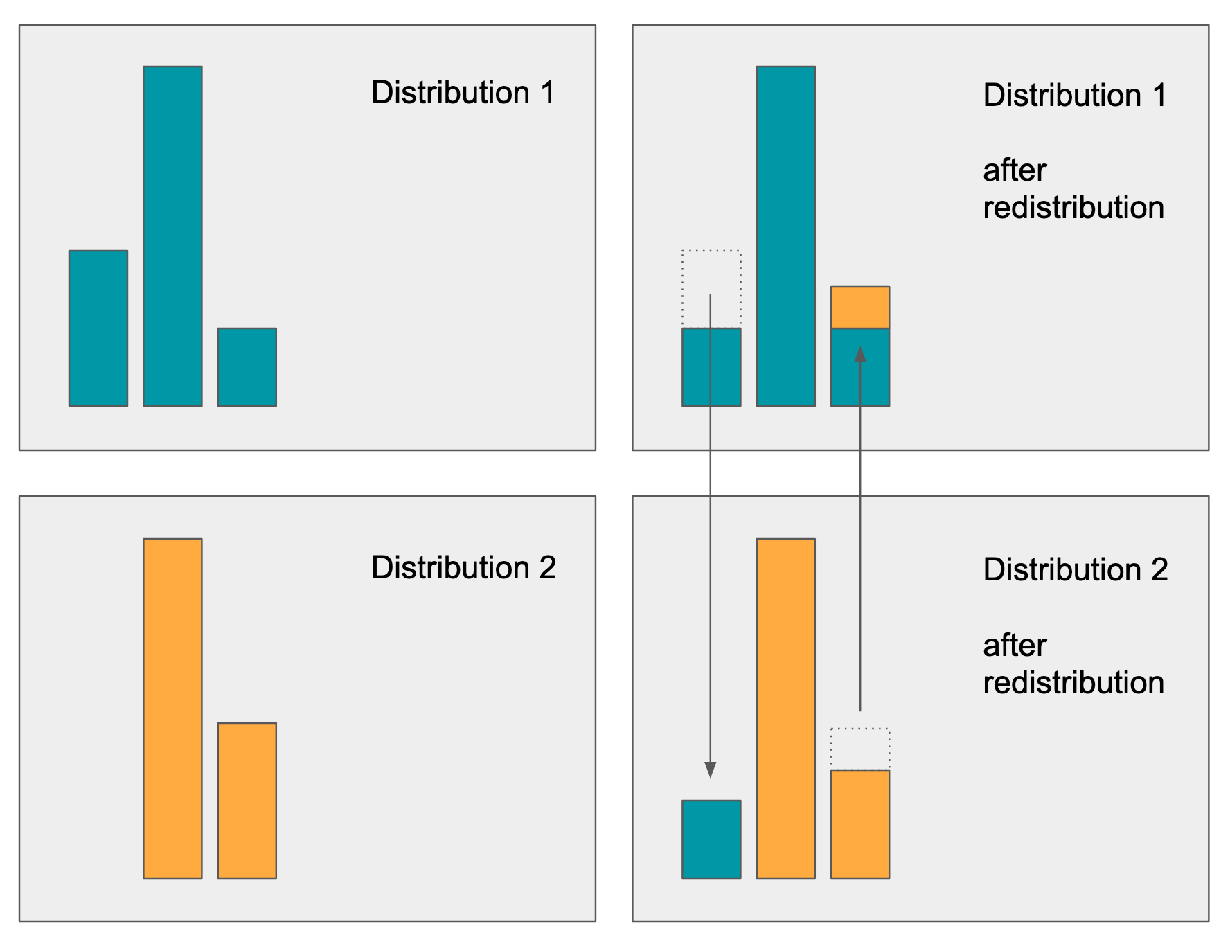
The amount of mass redistribution (and distance travelled) is a good representation as to how different any two distributions are, and is applicable to both univariate and multivariate distributions.
Greedy algorithm 1
The algorithm is as follows:
- rank features by degree of separation between \(p(x_i)\) and \(p(x_i\, \vert\, f(x) = c)\), for each class c
- select highest ranked feature to initialize list of features
- iteratively select K-1 features as follows:
- select next highest ranked feature
- evaluate correlation of feature versus already selected features
- if maximum correlation > threshold (say 0.7), discard this feature
- once K features have been selected, done
def select_by_EMD (df: pd.DataFrame, labels: pd.Series, topk = 25, maxcorr = 0.70):
    names = df.columns.values
    scores = np.zeros(names.shape[0])
    for i in range(names.shape[0]):
        feature = names[i]
        xprior = df[feature]

        # we assume binary classes in this case
        xcond0 = df[feature].loc[labels == 0]
        xcond1 = df[feature].loc[labels == 1]

        w0 = (labels == 0).sum() / float(labels.shape[0])
        w1 = (labels == 1).sum() / float(labels.shape[0])

        d0 = wasserstein_distance(xprior, xcond0)
        d1 = wasserstein_distance(xprior, xcond1)
        scores[i] = w0 * d0 + w1 * d1

    indices = np.argsort(scores)[::-1]
    features = names[indices]
    importance = scores[indices]

    selected_features = [features[0]]
    selected_importance = [importance[0]]
    for i in range(1, names.shape[0]):
        feature = features[i]
        v = df[feature]
        corr = df[[feature] + selected_features].corr().iloc[1:,0].max()

        if corr <= maxcorr:
            selected_features.append (feature)
            selected_importance.append (importance[i])
        if len(selected_features) == topk:
            break

    return pd.DataFrame({
        "order": np.arange(len(selected_features)),
        "feature": selected_features,
        "importance": selected_importance }).reset_index(drop=True)

# select the top 10 features from feature `xtrain` against labels `ytrain`
selected = select (xtrain, ytrain, topk = 10)
Improvements
- look at 2 or 3 dimensional conditional distributions such as \(p (x_i x_j x_k \, \vert \, f(x) = c)\)
- This would allow us to determine subspaces that are jointly explanatory where a single feature may be less so. I would have to think carefully as to how to compare these.
- Rationalize correlation between variables
- how do distances interact for highly correlated variables; can we factor out overlapping sensitivities?
For now have use a heuristic algorithm to deal with the correlation overlap, and also avoided the sub-space considerations.
Conclusions
In this post I did not compare the “goodness-of-rank: of this method versus other methods (this is quite hard to do objectively). However, in practice have found this method:
- at least as good or better than Random-Forest Gini based feature selection
- has a sound information-geometric basis
- provides good intuition as to how / why features were selected