Information In Volatility Structure [1]

I’ve developed signals based on the “spot” market, but had not really explored the options market as a source of information. In particular want to look at discrepancies in option demand / pricing that may relate to future returns or risk. In scenarios where there is an expected dislocation in price, there may be more demand for calls vs puts or vice-versa. Buying pressure on puts or calls will tend to impact the option price (and therefore implied vol), much as unbalanced buying / selling impacts price in the “spot” market.

Towards this end I want to look at measures of the shape of the implied vol (IV) curve for one or more given constant maturities. The most obvious place to start is by looking at volatility. One such common measure is:

      

where would evaluate this measure over time for a specific constant maturity. I will also be looking at other attributes of the vol surface, but the above is probably a good starting point. Expect that there will be a good amount of noise day to day, so will need to look at denoised measures of skew.

Given the need to look at a constant maturity, we will be “walking” the volatility surface over time, measuring vols in between observable expiries. Hence will need to build a volatility surface on moneyness vs time, allowing us to project IVs for any given moneyness / strike / delta and expiry.

As with building interest-rate curves, there are certain constraints with respect to arbitrage that should be observed in building a volatility surface, but the rest is more of an art than a science. As am not going to be using the vol surface to price exotic options, rather focusing on an approach that produces a smooth fit through noisy data. After evaluating a number of different models, the SABR model seemed to be the right combination of expressiveness and parsimony.

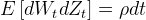
While the SABR model may not be as sophisticated as some of the more complex stochastic volatility models it is fairly easy to calibrate and reason with. The SABR model is a stochastic vol extension of the CEV model. The CEV model was perhaps the first to express a relationship between asset price level and volatility, where volatility has a tendency to inncrease as the asset price decreases. The beta and skew parameters of the CEV model allow for a variety of distribution configurations. The SABR model goes further, allowing for separate, correlated, evolution of both the forward price and volatility over time, expressed as:

      

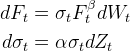
where the stochastic processes are correlated in the following manner:

      

To calibrate a section of the surface, along the strike / moneyness axis, we then determine appropriate parameters of alpha, beta, nu, and rho (often with a fixed value of beta), that determine a least-squares fit between market IVs and modeled IVs. An approximation for IV is given by:

      

One can then use multivariate gradient descent to determine a least-squares fit beteen observed market IV and SABR-implied IVs. Using the Levenberg-Marquardt algoritm paired with an error function, and reasonable initial starting parameters, can regress towards an error minimum.

Problems

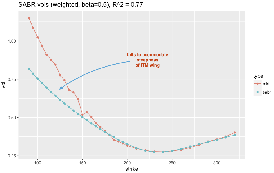
Given only 3 degrees of freedom (typically with fixed Beta) and a log polynomial structure in F, the SABR model cannot express the full variety of curvature seen in empirical smiles. Below is a case in point, where in order to accommodate the steep smile, the curvature near the ATM causes the function to undershoot the market vols (observe the undershoot between 220 and 240 strikes). The market vols should be flatter near the money and steeper further away.

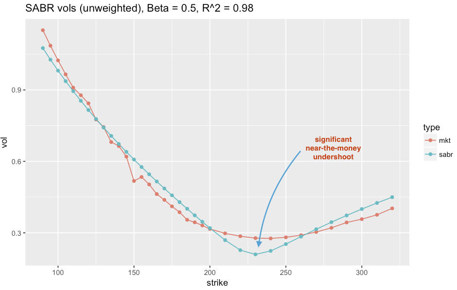
Speaking to a friend who trades FX derivatives, indicated that practitioners have similar issues, where SABR often implies a steeper vol surface near-the-money than the market trades. This is an artifact of insufficient explanatory capability, where the model cannot fully resolve both the curvature of the steep wings and the flatter section near the money. As the wings are steep, minimizing their error will tend to dominate a least-squares fit, at the expense of “flatter” regions of the curve that cannot be accomodated by the log polynomial structure.

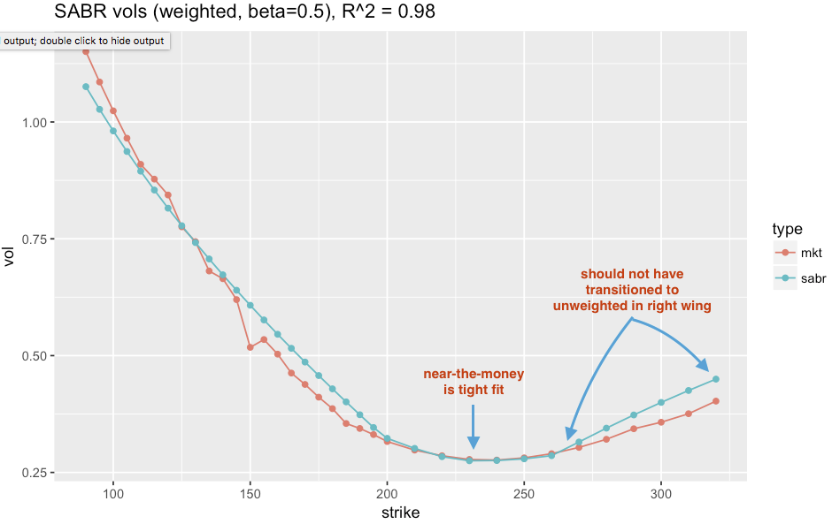
Given that most of the trading volume occurs on near-the-money strikes, thought could rectify the lack of fit near-the-money by using a weighted least squares solution, adjusting the error function to weight the square error by the trading volume at a particular strike. This improve the accuracy of the near-the-money strikes significantly, but the SABR function does not have enough degrees of freedom to overcome the steep curve required for the deep-in-the money strikes (below 200).

Neither of these approaches was sufficient for my purposes. My variant of weighted SABR often provides good resolution between 15 to 75 delta but with poor resolution in the wings. Conversely, the unweighted SABR usually provides the best estimation of the wings, but with poor resolution on the near-the-money strikes.

A Heuristic Approach (1st pass)

I took the approach of computing both of the weighted and unweighted SABR model and blending on transition points on the wings. I use a linear blend between the weighted and unweighted over a range between the near-the-money portion (weighted) and the deep in/out of the money portion (unweighted). The first implementation below, started a 5 delta transition at 15 delta and 90 delta points, from the weighted to unweighted out to the wings. This improved on the degree of fit, providing needed precision at the near-the-money strikes and preserving overall shape in the deep in/ou of the money wings:

However, one can seen that the original weighted calibration (in the prior section) does much better beyond the 260 strike. A better approach would be to use the weighted SABR for the near-the-moneys and extend its influence until it is clear that a blend into the unweighted SABR would be superior. For example, the “optimal” fit might be one where the weighted curve runs between 175 and 325+ and the unweighted curve is blended in below 175.

A Heuristic Approach (2nd pass)

Computing the error of each model versus the market vols:

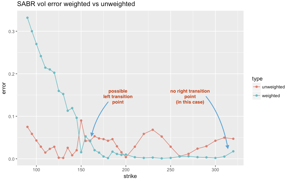
We can see that the error of the weighted SABR is lower for a region between 160 and the end (325). The new algorithm makes use of the error function, determined the “best” left and right transition strikes by observing where the error function shows lower error for K consecutive points (I use K = 3). The requirement for K consecutive points avoids most data noise. Here is the estimation of the vol function with this new approach:

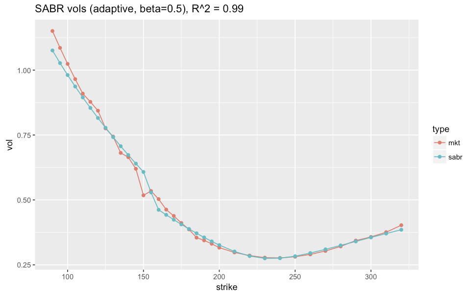
The overall fit is much better then any of the prior approaches, with a 99% R^2. While the continuity and direction of the curve is maintained on the left wing, there is a flip in convexity at the point of transition. That said, find this curve preferable to the above alternatives.

Final Thoughts

The solution is far from perfect. One would hope to use a model with enough degrees of freedom to express the full repertoire of smiles. I have not fuly investigated all of the stochastic volaility models, though expect some will do quite a bit better here, though at the cost of much greater complexity. Given that my goal is to smooth over data anomalies (for example the 150 strike in the above example), the explanatory shortcoming does not pose a problem.

I will be evaluating 10 - 20 years of equity option data (with adjustments for dividends). Will post more about what I find in coming weeks.

Addendum

The analysis and graphs above were evaluated with fixed Beta = 0.5 (and therefore only 3 degrees of freedom). Allowing the solver 4 degrees (with free Beta) reduced the curvature issues noted above, howeever did not eliminate them. The adaptive algorithm still provides superior fit to either the unweighted or weighted SABR algorithm with 4 degrees of freedom.