Why ML → Finance is Hard (2 / 4)
Label noise and what we can do about it
Following on from the prior post, want to discuss the repercussions of the low signal / noise ratio and how it effects:
- labeling / mis-labeling
- patterns unsupported by features
How does this manifest and what might we do to ameliorate the issues it poses.
Introduction
Financial timeseries appear to have a very low signal to noise ratio, where the variance (the power of the noise frequency) can be higher than the power of the overall signal. There are many different ways to quantify the S/N ratio of a financial timeseries, but will not pursue here.
Price uncertainty is a function of limited information. If we knew or could deduce the individual decision making and information state of each market actor, we would could have certainty about the next action of each participant. This would still not be enough to predict future prices far forward, unless we could also model the future states of exogenous information influencing market actors. While I am aware of and have been involved in limited modeling of actors in the market (for example market makers model how groups of traders (clients) or specific clients behave), future event prediction would require a super-human AI that could predict our ecosystem.
Given our lack of capability to know or predict the actions of individual actors, we have to take on a stochastic view of the market where the following exist:
- underlying price direction
- substantial noise added to the price direction by differing views of price discovery (or due to purposeful obfuscation)
- supply and demand dynamics which temporarily disrupt longer term price direction
- shocks and regime change
The label noise problem
The preponderance of machine learning models are supervised (i.e. labeled classifiers or regressors). Such models take on the form:
\[\hat{y} = f(\vec{X}) + \epsilon\]where we train the function f(X) to minimize a loss function and a complexity tradeoff, for example:
where \(L(y,\hat{y})\) is the loss function and \(\lambda ||x||_1\) is the complexity penalty. There are many different formulations of the optimisation. I recommend this article on loss functions as an overview on the types of loss functions typically deployed. As for the optimisation, may look quite different depending on ML algorithm and structure. Decision tree models, for example, are quite different from SVM and deep learning in loss function approach.
If our labels (the labels provided in training) have high error, we have biased the model towards that error. A 50% error rate in our labeling would certainly result in a model that is as good as random. However, much lower error rates will tend to be enough to derail a ML model:
- trading opportunities are often the minority label
- (+1 for enter may be 1/3rd or 1/4 of all labels, in the binary classification case)
- certain feature / label pairs may be emphasized much more strongly in the model
- (for example due to higher variance of particular feature vectors)
- features have their own noise, contributing to degradation of OOS model performance
Label Noise: Digging In
Lets get a sense of the error presented in daily returns relative to a smooth projection of forward returns in our prior example. Recall that our labels were based on the 5 day return being >= 50bps. To simplify the analysis, lets consider the noise in daily returns relative to smoothed forward cumulative returns (in bps).
...
prices = pd.Series(bars["Adj Close"].values.flatten())
cumr = np.log(prices / prices.iloc[0]) * 1e4

def smooth (y: pd.Series, bandwidth: float):
    x = np.arange(0, cumr.shape[0])
    return pd.Series(lowess(y.values.flatten(), x, frac=bandwidth)[:,1].flatten())

smoothr1 = smooth(cumr, 0.002)
smoothr2 = smooth(cumr, 0.01)
error1 = cumr - smoothr1
error2 = cumr - smoothr2

stat1 = np.abs(error1).median()
stat2 = np.abs(error2).median()
...
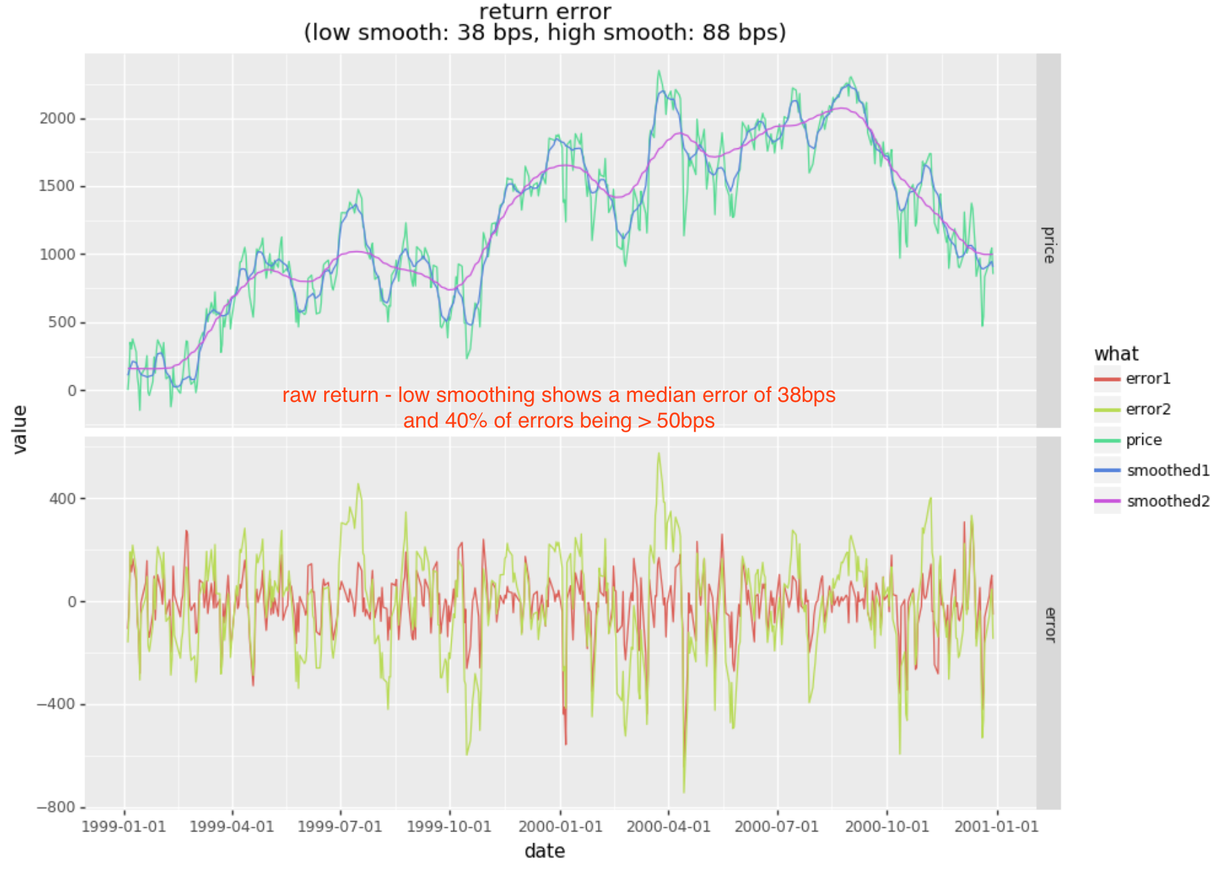
The low smoothing (smoothing1) is fairly light smoothing with an approximate period in line with the 5day return direction. Note that the median error is 38bps and that 39% of these errors exceed 50bps (whereas the remaining 61% are below 50bps). An error rate this high will derail any model targeting return based labels.
Feature Noise: Digging In
As you can imagine, features based on prices can also exhibit similar noise. Let’s cheat a bit and see what happens if we smooth prices used for both features and labels, removing the label and feature noise. Note that this will not result in a valid strategy as the smoothing used above is global and therefore has a lookahead bias. However the difference in OOS outcome should be significant if we denoise.
...
smoothr1 = smooth(cumr, 0.001)
smoothr2 = smooth(cumr, 0.002)
smoothr3 = smooth(cumr, 0.005)

# create features
df = pd.DataFrame({
    "rsi.1": talib.RSI(smoothr1, timeperiod=14),
    "rsi.2": talib.RSI(smoothr2, timeperiod=14),
    "rsi.3": talib.RSI(smoothr3, timeperiod=14),
    ...
})

# create { 0, 1 } labels, where 1 means smoothed 1day return >= 20bps
df["rfwd"] = df["roc1.1"].shift(-1)
df["label"] = (df.rfwd >= 0.20) * 1.0
...

icut = int(df.shape[0] * 0.70)
training = df.iloc[:icut].dropna()
testing = df.iloc[icut:].dropna()

clf = RandomForestClassifier(n_estimators=500, random_state=1, n_jobs=-1)
model = clf.fit (training[features], training.label)

pred_train = model.predict(training[features])
pred_test = model.predict(testing[features])
In this scenario we now get an OOS precision of 72% instead of 47% precision in the prior model. If it were not for the lookahead bias in smoothing, this would lead to a very profitable strategy.
| / | Positive | Negative | Accuracy |
|---|---|---|---|
| Positive | 408 | 159 | 72% |
| Negative | 209 | 851 | 80% |
Dodging the problem
Without solving the noise problem there are ways of avoiding the “labeling problem”, for example:
- unsupervised learning (without a label objective)
- examples of this include HMM, KNN, etc
- regression
- this is quasi-labelled in that maps to (noisy) outcomes, but does not have quantized outcomes as with classification
- EA (genetic algorithms and genetic programs)
- one solves for an overall performance objective rather than targeting labels
Of course using any of these means one has reframed a problem in a very different way. There are many times where classification makes the most sense, and the above are not especially applicable.
Partial Solutions
There has been some limited exploration of noisy labels in the literature (here is an example),
though one rarely sees direct support for class-conditional noise loss functions in libraries such as sklearn.
The loss approach discussed in the linked paper assumes a consistent noise distribution across the labels. Whereas
we should expect that our label noise varies across time with market volatility (the conditional noise distribution changes
over time).
There are some heuristic approaches one can take:
- the most obvious, remove noise with pre-smoothing
- Given that noise exists in both labels and features (where removing feature noise often cannot be removed without lookahead bias or alternatively lag), pre-smoothing only addresses label noise and not feature noise
- use a classification algorithm that allows weights, weighting the samples based on expected label noise
- this limits the ML algorithms we can use and also means our model fails to predict well in higher volatility situations
- the lower weight samples may also be of more interest in trading, defeating the purpose
A more interesting heuristic approach (which I have used successfully) attempts to circumvent feature and label noise simultaneously by using a 2 stage approach to classification:
- use a model trained on original labels to generate new labels
- some % of these labels will be our given labels and some % relabelled to an alternative class
- retain TP, TN, and FN, however remap FP → 0
- do this on N folds within the training set until the whole training set is relabeled
- train a new model based on the generated / modified labels
- I found that this improves precision, removing the impedance where TP’s could not be achieved with the original labeling
Sample Code (for resampling labels with a RF)
def relabeled(X: pd.DataFrame, y: pd.Series, nfold = 10):
    w = X.shape[0]
    cuts = np.arange(0,w+1,w/nfold, dtype=int)
    cuts[-1] = w

    newlabels = np.zeros(w)
    for i in range(0,cuts.shape[0]-1):
        xtesting = X.iloc[cuts[i]:cuts[i+1]]
        ytesting = y.iloc[cuts[i]:cuts[i+1]]

        xtraining = pd.concat([X.iloc[:cuts[i]], X.iloc[cuts[i+1]:]])
        ytraining = pd.concat([y.iloc[:cuts[i]], y.iloc[cuts[i+1]:]])

        clf = RandomForestClassifier (n_estimators=500, random_state=1, n_jobs=-1, class_weight='balanced')
        model = clf.fit (xtraining, ytraining)
        ynew = clf.predict(xtesting)

        TP = (ynew == 1) & (ytesting == 1)
        FP = (ynew == 1) & (ytesting == 0)
        FN = (ynew == 0) & (ytesting == 1)
        TN = (ynew == 0) & (ytesting == 0)

        precision = TP.sum() / (TP.sum() + FP.sum()) * 100.0
        print ("[%d/%d] precision: %1.1f%%" % (i+1, cuts.shape[0]-1, precision))

        ynew[FP] = 0.0
        newlabels[cuts[i]:cuts[i+1]] = ynew

    return newlabels
Alternatives
There are a variety of methods described here “Confident Learning”. I have not found these methods to be as useful as the heuristic above, probably because of the focus on labels versus the combined behavior of noisy features and noisy labels.
Conclusions
I am still very unsatisfied with the handling of this problem. I think the optimal solution will lie in creating machine learning algorithms that explicitly allow one to parameterize feature and label noise across the data set. Will think further on how this should be structured. Would love to get pointers from anyone that has dealt with these problems.
In the next post I will try to tackle lack of feature vector independence.