Arbitrage In DEFI (p2)

As mentioned in my prior post Arbitrage in DEFI (p1), have been building and improving a MEV strategy in DEFI to perform both atomic and non-atomic arbitrage, backrunning, liquidations, etc. In this article we continue to focus on algorithms to detect and optimise arbitrage paths through the pool graph.

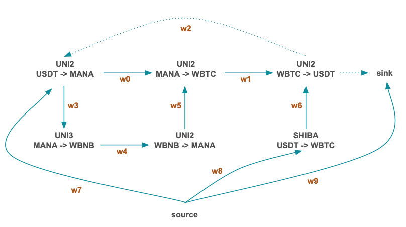
Let us consider a simple graph of possible flows between 6 pools:

Bute-force approach (for small graphs)

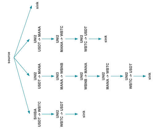
For smaller graphs, we can avoid evaluating a complex optimisation by simply doing a DFS traversal to determine all possible acyclic paths from source -> sink:

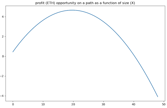
Given all possible paths we can evaluate the optimal flow through each path in order to maximize outcome. As we put more flow (size) through a given pool, we are penalized with an increasingly worse price and outgoing size. Hence the payout for a profitable path will be a concave function such as this:

An optimisation on the path determines the size of the flow through the path that maximizes this function. For a small enough graph we could generate all such paths and maximize each one with a simple solver. However, the approach of generating all acyclic paths grows combinatorially and is not feasible for a large graph.

Optimisation

We want to find the weights through this graph such that the (outgoing - incoming) flow from source -> sink (our wallet) is maximized. We can frame this problem graphically as a max-flow problem where we:

Note that the node transfer function (or amount of flow output for a given input) is as follows for a Uniswap V2-like AMM:

Quasi-Convex Optimisation

In the paper Optimal Routing for Constant Function Market Maker, Angeris et al showed an elegant approach to determine the optimal amounts to be traded across a collection of pools maximizing some utility function (for example maximize output of ETH) within the constraints of CFMMs.

where:

• $(\Delta_i, \Lambda_i)$ is the amount in and amount out for the ith pool
• $A_i$ indicates the adjacency matrix between tokens
• $\phi_i(*)$ is an expression of the constant product reserve constraint
• $U(\Psi)$ is the utility function, for example: $U(\Psi) = prices_{mkt} \times \Psi$, maximizing market value of net output

The setup of this problem works beautifully on small to medium sized acyclic graphs, but is not stable or becomes overwhelmed in the following contexts:

• graphs with cyclical feedback
  • the possible sub-graphs present different discontinuous gradient functions
• large graphs with hundreds of thousands of edges
  • many of these algorithms have complexity $O(n^3 log(1/\epsilon))$, which does not scale for large sized problems in the 10K+ range

We can make this approach workable if we can significantly reduce the graph, focusing on profitable neighborhoods, and remove cycles prior to applying the optimisation (I may elaborate on this in a subsequent post).

Max-Flow Optimisation (for acyclic graphs)

If the graph is acyclic we can efficiently solve the max-flow problem as follows:

1. determine a function to resolve flows given a weight vector (essentially a graph traversal)
2. determine the gradient of the network with respect to weights
3. determine objective function (for example maximize flow into sink node)
4. use L-BFGS-B to solve for the objective

This works well, but does require that the graph has no cycles. With cycles a continuous gradient cannot be determined due to the discontinuity of an edge / cycle being in the graph or excluded. If the number of cycles is limited can evaluate each graph alternative separately. I have an implementation for this that arrives at the global optimum in approximately $O(n\, log(n))$ time.

Heuristic Optimisation

As mentioned above convex optimisation approaches have issues in tackling the complexity and scale of these graphs. Heuristic optimisation algorithms such as differential evolution (DE) and simulated annealing are well suited to finding a global optimum in the presence of:

• multiple local minima
• discontinuous solution surfaces
• mixed integer and continuous domain

Neither of these solutions is guaranteed to arrive at the absolute maximum (minimum) due to their stochastic nature, however can get quite close or alternatively converge arbitrarily close to the optimum with increased iteration.

Differential Evolution is more capable than Simulated Annealing in terms of being better able to explore the solution space. This benefit comes at the cost of requiring more computation, at least in early iterations, however. DE is a special case of a genetic algorithm, one where new individuals from generation to generation are expressed with gradient aware operators. SA has some similarities to DE in the sense that the parameter vector is perturbed in each successive generation, however one can easily get stuck in some part of the domain depending on the starting point of the simulation. DE is able to continue to explore the domain, though will tend to do so less in successive generations.

I found that differential evolution was consistently able to arrive close to the global optimum, whereas simulated annealing might find a local optimum 50% of the time. SA could be adjusted to use a sampling (multi-simulation) approach and take the maximum over those simulations.

Bellman-Ford Optimisation

In the BF construction of the problem, we do not solve for max-flow directly, rather look for minimum paths through the graph where the weight is the $-log(price_i)$. If we circuit from, say, WETH -> … -> WETH and have a negative cumulative path, then have found a profitable path.

The problem with BF algorithms are that they:

• assume that price remains constant with size
  • so have to test for profitable paths on some unit size, later requiring a secondary optimisation to determine appropriate size
• algorithm cannot handle cycles
  • there are various heuristic approaches to trimming the graph in the presence of a cycle, but does not lead to optimal solutions. It can still provide viable, if not optimal, paths however.

Example

We want to find profitable paths through the following, given a source with 20 WETH:

• Uniswap V2: ETH <-> USDT
  • reserves: 20100184, 10000, fee: 30bps
• Sushiswap V2: USDT <-> ETH
  • reserves: 20020000, 10830 fee: 30bps
• Uniswap V3: USDT <-> ETH
  • reserves: 20000000, 11040, fee: 30bps
• Shibaswap V2: USDT <-> ETH
  • reserves: 23000000, 10000, fee: 30bps
• Sushiswap V2 USDT <-> BTC
  • reserves: 101, 5000000, fee: 30bps
• Sushiswap V2: BTC <-> ETH
  • reserves: 100, 3518, fee: 30bps

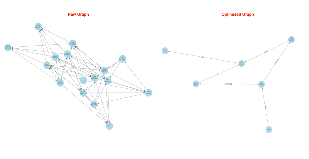
Here is the raw graph without optimisation and the graph post optimisation (where we have identified the optimal flow through the graph from source -> sink):

Solving with Differential Evolution

Differential Evolution is not the most efficient approach, however is one of the simplest and one that can achieve global optimum. In a subsequent post I will discuss a hybrid approach to reduce the size of the graph and allow for more economical solutions.

The approach to solving the max-flow problem with DE is as follows:

1. determine a function to resolve flows given a weight vector
   • this is essentially a graph traversal where we evaluate incoming flows x weights and compute outgoing flows
   • we also terminate and zero-out cycles when detected
2. write a function to enforce constraints $\sum_i w_i \le 1$ and also sparsify weight vectors
   • for sparsification I use $\bar{w}^k / \sum_i w_i^k $, pushing values towards 0 or 1
3. determine an objective function
   • maximize sum of incoming flows into sink node
4. write or use an existing differential evolution algorithm
   • python scikit has a differential_evolution function
   • rust has crates for this as well differential_evolution and metaheuristics_nature
   • I’ve written a DE / GA implementation for C++ as well

Code

Realistically one will implement optimisation in Rust or C++, however for a more concise presentation am providing some python code snippets here for the DE approach.

Pool

This class defines functionality for a Uniswap V2-like pool or top-of-book V3 pools. Here is the output function defining amount out for a given amount in, according the CFMM constraints:

def amount_out(self, amount_in: float) -> float:
    """
    Compute the amount of money outgoing given incoming amount in the pool.  The amount in should be in
    the units of cin.
    """
    if self.reserve0 >= 0 and amount_in > 0.0:
        k = self.reserve0 * self.reserve1
        gamma = 1.0 - self.fee
        return self.reserve1 - k / (self.reserve0 + gamma * amount_in)
    else:
        return amount_in

Resolving Flows

We want to determine flows through the graph, given a weight vector (where the weights define the % of flow per edge):

def resolve_graph(self, weights, amount_in):
    """
    Resolve the graph for given weights and amount in
    """
    def resolve_flow(weights: np.array, node: Pool, seen: set, eps=1e-4) -> float:
        if node.id in seen:
            return node.outgoing if not np.isnan(node.outgoing) else 0.0
        if not np.isnan(node.outgoing):
            return node.outgoing

        seen.add(node.id)

        # normalize incoming edges to sum <= 1 and sparsify
        incoming_edges = node.incoming_edges(self.G)
        self.normalize_and_sparsify (incoming_edges)
        
        # determine amount of inflow
        inflow = 0.0
        for edge in incoming_edges:
            iedge = self.edge_to_idx[edge]
            ancestor = self.pools[edge[0]]
            w = weights[iedge]
            if w > eps:
                out = resolve_flow(weights, ancestor, seen)
                inflow += w * out
            else:
                out = 0.0

            # clamp near-zero weights to 0
            if out == 0.0:
                weights[iedge] = 0.0

        node.outgoing = node.amount_out(inflow)
        node.incoming = inflow

        return node.outgoing

    seen = set([])
    for node in self.nodes:
        node.reset()
    for node in self.nodes:
        resolve_flow(weights, node, seen)

Objective

Our objective function is simple:

1. resolve flows across graph for a given weight vector
2. determine output flow vs input flow

def objective(weights: np.ndarray) -> float:
    """
    Maximize profit as: `flow reaching sink` - `amount in` (as a minimization problem)
    """
    self.resolve_graph(weights, amount_in)
    return -(self.pools[sink].incoming - amount_in)

Optimisation

We then call our DE optimiser:

result = differential_evolution(
    func = objective,
    bounds = ranges,
    maxiter = maxiter,
    popsize = population,
    disp = True,
)
self.weights = result.x
self.profit = -result.fun - amount_in

Upcoming

There is no entirely satisfactory solution for the optimisation problem in that:

1. the presence of cycles invalidates a number of optimisation approaches
2. the scale of the problem is such that traditional optimisers cannot solve efficiently
3. heuristic optimisation can determine the global maximum +/- the stochastic nature of the algorithm

In a subsequent post will elaborate on an approach to reduce the problem significantly, making more amenable to a variety of these approaches.