Denoising a signal with HMM

Most signals I deal with are noisy, reflecting noise of underlying prices, volume, vol of vol, etc. Many traditional strategies built on such indicators might either:

• use signal to scale into position
  • such approaches have to deal with noise to avoid thrashing, adjusting position up and down with noise
• consider specific levels of the signal to signify a state
  • for example: long {+1}, short {-1}, neutral {0}

Pictured below is an example of a noisy signal that detects downward momentum. The goal is to signal 1 when in downward momentum and 0 when not. A simplistic approach might be to set a threshold and map the raw signal to 1 when above threshold andto 0 when below the threshold.

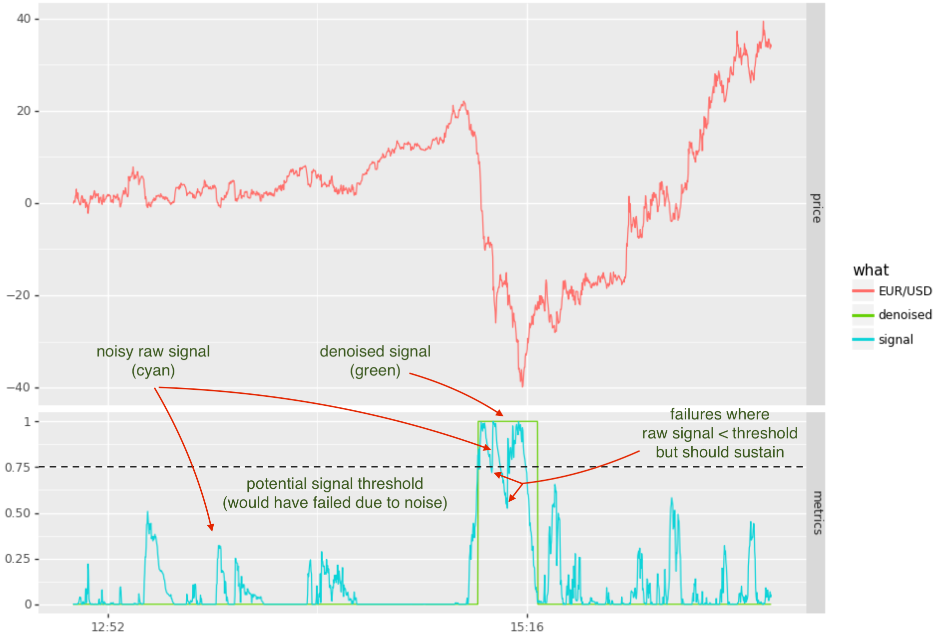
In the above scenario, there is no threshold level that would avoid unwanted oscillation between 0 and 1 states. For example, with the threshold set at 0.75 there are 2 incursions below the threshold (which would be mapped to state 0). Trying other thresholds, such as 0.5, avoiding noise during the momentum period, but would encounter noise thereafter.

The denoised signal (pictured as the green line), makes use of a hidden markov model (HMM). Have used this for the past 10 years or so, so thought to share the approach here.

A Solution

In the application above we are interested in assigning states (or levels) +1 and 0, removing the noise from our signal. Let’s consider a common scenario where we want to assign { Short, Neutral, Long } states to a noisy signal.

State System

To do this can construct a 3 state system and assign transition probabilities, for example probability of transitioning from Long to Short, Neutral to Long, remaining in the same state, etc.

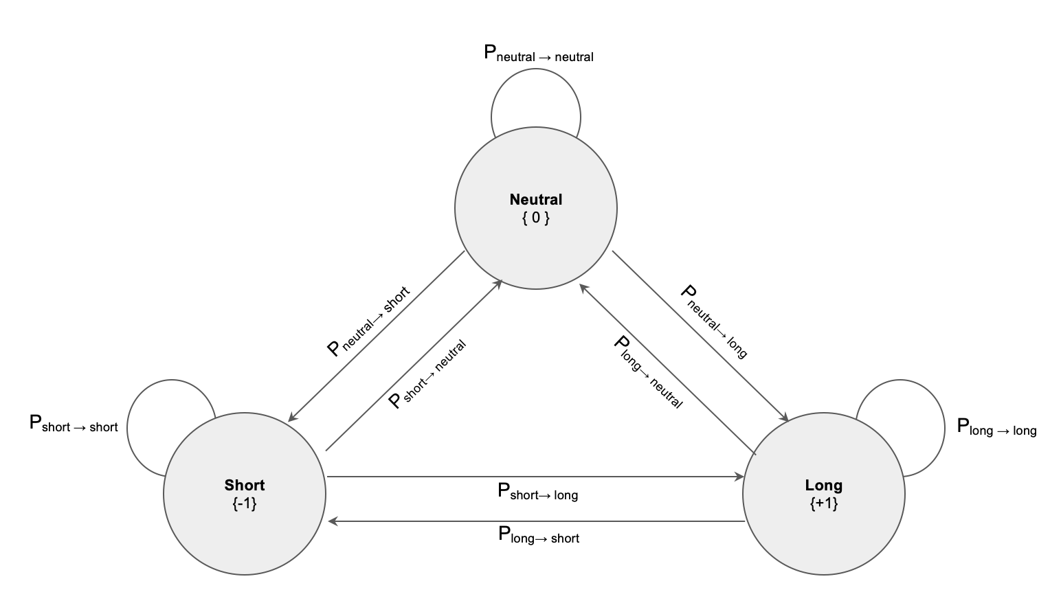
One can think of the same state probability as defining the “stickiness” to a given state, and resistance to noise that might otherwise cause us to transition to another state. For example if we assign a high probability to \(P_{short \rightarrow short}\), and a corresponding lower probability to transitions out of that state, we will be able to ride more noise without transitioning to another state.

The state system above gives us a transition matrix:

Note that the probabilities must sum to 1 across each row, i.e. for transition matrix M: \(\sum_j M_{i,j} = 1\). If one wants to define the denoising model in terms of “stickiness” to same state, then can determine the probabilities for the 3-state transition matrix as:

and for a 2-state matrix as:

Observation Distributions

Next we need to consider how the (noisy) signal is mapped to these states. The approach taken by HMM is to introduce an observation distributions \(p(y \vert x)\), where \(y\) are our observations (the raw signal in this case) and \(x\) is the particular “hidden state”.

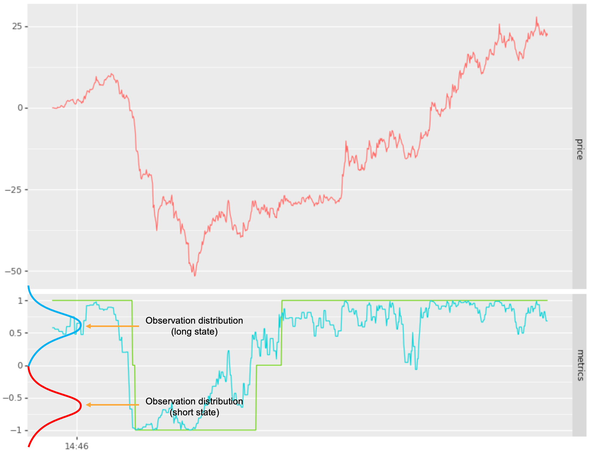
Our next step is to design an observation distribution for each state, providing separation such that the likelihood of \(p(y \vert x = s_i)\) versus \(p(y \vert x = s_j)\) are significantly different for signal values that should be mapped to state \(s_i\) versus state \(s_j\) respectively. In the example below I map a noisy signal into 2 states { long, short }, using normal distributions:

• long state: \(p(y \vert x = long) = N(+0.65, \sigma)\) or
• short state \(p(y \vert x = short) = N(-0.65, \sigma)\).

See below:

Tying it together with HMM

The observation distribution provides us with \(p(y \vert x = s)\), but what we are looking for is \(p(x = s \vert y_n, y_{n-1}, .. y_0)\), i.e. the probability of being on state “s” given the observation sequence (our noisy signal), \(y_n, y_{n-1}, .. y_0\).

The HMM model ties the transition probability matrix \(M\), our observation probability distributions \(p(y \vert x = s)\), and state probability priors \({ \pi_{s = short}, \pi_{s = neutral}, \pi_{s = long} }\) into a model which determines the most likely state as we proceed along the sequence of observations. (The priors are typically determined as the frequency of each state such as 1/3, 1/3, 1/3).

As concisely described here, at each time step in the sequence we compute the likelihood of being on state \(x_t = s\) as:

where \(p(x_t \vert x_{t-1})\) is our transition probability across all possible combinations of states as defined by \(M\) and \(p(y_t \vert x_t)\) is our observation distribution for given state at \(x_t\). For t = 0, \(\alpha_t(x_t)\) is defined in terms of the prior distributions for each state as \(p(y_0 \vert x_0 = s) \pi_s\)

The above is decomposed into a dynamic programming problem. The algorithm in pseudo code is as follows:

# initialize time step 0 using state priors and observation dist p(y | x = s)
for si in states:
    alpha[t = 0, state = si] = pi[si] * p(y[0] | x = si)

# determine alpha for t = 1 .. n
for t in 1 .. n:
    for sj in states:
        alpha[t,sj] = max([alpha[t-1,si] * M[si,sj] for si in states]) * p(y[t] | x = sj)     

# determine current state at time t
return argmax(alpha[t,si] over si)

Note that the above would be restated in log likelihood space to avoid underflow and avoid having to compute the distribution CDFs.

Filtering (summary)

In summary, the approach to mapping a Long / Short signal or alternative configuration of states is to:

• define the observation distributions in a way that separates states in the signal domain
• define a transiton probability matrix controlling “stickiness” (amount of state transition noise)
• define priors (typically the frequency one expects for each state)
• use the forward viterbi model to determine the state sequence \(x_{t:0}\) as a function of observed raw signal sequence \(y_{t:0}\)

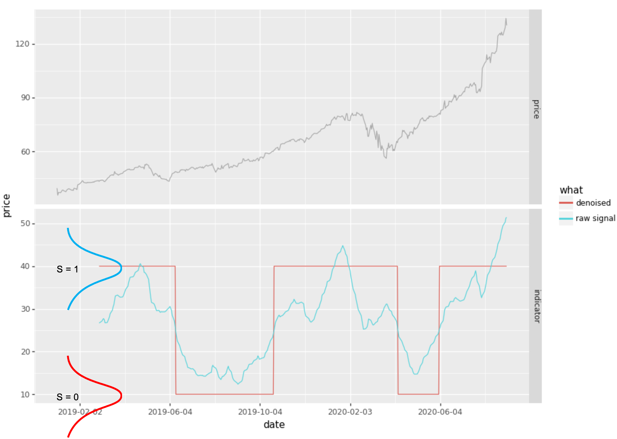
Here is an example (which I did not attempt to optimise):

from tseries_patterns.ml.hmm import HMM2State
from tseries_patterns.data import YahooData
from talib import ADX


# get price bars
aapl = YahooData.getOHLC("AAPL", Tstart='2019-1-1')

# compute our raw signal (not a very good one, FYI)
rawsignal = ADX(aapl.high, aapl.low, aapl.close, timeperiod=20)

# denoise signal
hmm = HMM2State (means = [10, 40], ss_prob = 0.9999)
## predict 0 and 1 states, rescaling to 10, 40 to align with scale of ADX
denoised = 10 + hmm.predict(rawsignal.dropna()) * 30

# plot
...

The above HMM2State class explicitly defines:

• the transition probability matrix:
  • \(i = j \rightarrow 0.9999\) and
  • \(i \neq j \rightarrow 1 - 0.9999\).
• the observation distributions as:
  • \(S_0 = N(\mu = 10, \sigma_{default})\) and
  • \(S_1 = N(\mu = 40, \sigma_{default})\).
• the prior probabilities as \(\pi_i = \frac{1}{2}\)

The forward viterbi method is then used to determine the states in the hmm.predict() call. HMM2State is a simple wrapper around the underlying scikit hmmlearn implementation that defines the model, bypassing the fit() stage.

Alternatives (that don’t work well)

A typical approach with HMM involves using the forward-backward algorithm to automatically determine:

• transition probabilities
• observation distributions
• priors

For example:

from hmmlearn.hmm import GaussianHMM

rawsignal = ...
model = GaussianHMM(n_components=3)
model.fit (rawsignal)

states = model.decode(rawsignal)

While this will find 3 states, is unlikely not to have the desired filtering effect:

• the 3 observation distributions may be skewed by biases in the raw signal
• the transition probabilities are unlikely to represent the desired “stickness” and hence denoising desired.

In general you will achieve better results by defining the observation distributions and transition probability matrix yourself.