Feature Selection (1 / 3)
Introduction
I am often confronted with the problem of trying to reduce a high dimensional feature set to a, smaller, more effective one. Reducing dimension is important for machine learning models as:
- the volume of the “search space” grows exponentially
- at a minimum rate of \(2^{d}\) for binary categorical variables to a much higher exponential for continuous or n-ary categoricals.
- the joint-distribution of high dimensional empirical spaces tends to be sparse and ill-defined
- empirical distributions require data sample size in proportion to the volume of the space (exponential)
- cannot reasonably determine the joint distribution of sparsely supported spaces
- combinatorial explosion
- number of variable combinations can grow to an astronomical # (with n! growth)
- possible sub-space conditional distributions
Objective
Assuming we are pursuing a classification problem, the objective of feature selection should be to determine a feature subspace that maximizes discrimination between classes and minimizes model complexity. Alternatively, we can express this as a minimization of:
\[\DeclareMathOperator*{\argmax}{argmax} \DeclareMathOperator*{\argmin}{argmin} \newcommand\given[1][]{\:#1\lvert\:} \argmin_{ \vec{w} \in \{ set\, of\, all\, \left[ 0,1 \right]^d permutations \} } \sum_{i \in n} loss( f(\vec{w} \cdot \vec{x}_i), y_i) + penalty(\vec{w})\]where:
- loss function \(loss (f(\vec{x}_i), y_i)\) is the cost of mislabeling where \(f(\vec{x}_i) \ne y_i\)
- there are many different realizations of this function depending on whether is used for regression or classification and particular ML model. For example, for least-squares regression would simply be \(loss(\hat{y}, y) = (\hat{y} - y)^2\)
- penalty function \(penalty (weights)\) is a model complexity penalty
- L2 regularization imposes a \(\lambda \vec{w}^T \vec{w}\) penalty
- L1 regularization imposes a \(\lambda \sum_{i} \vert w_i \vert\), though refactored to avoid the discontinuity of the absolute value function.
Conceptually we could evaluate all (non-0 magnitude) permutations of the d-dimensional weight vector \(\vec{w}\) where weights are either 0 or 1, corresponding to enabling or disabling a feature. Some subset of features, expressed as 0 or 1 weights in \(\vec(w)\) will minimize the loss + complexity penalty.
Approaches
Here are some approaches:
- subspace projections from dimensionality d down to k, where k < d
- PCA, LDA, ICA, …
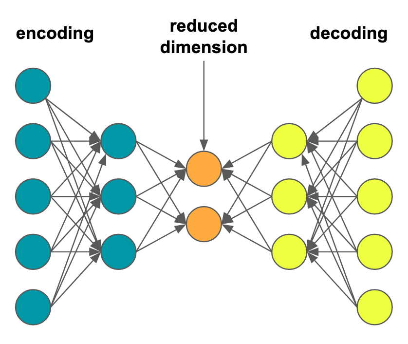
- auto-encoders: model (typically deep-learning) learns to reproduce d-dimensional features from lower dimensional k-dimensional synthetic features, in a feedback loop. The k-dimensional features are the dimensionally reduced output.
- ML model based, using ML model regularization to determine feature relevance
- random forest
- regression / classification with L1 regularization
- greedy
- iterative approaches where subsets of features are selected and evaluated against a particular model
- this is very data and model specific and likely to overfit.
- computationally infeasible to do exhaustively for high dimensional data sets
- information geometric approaches
- evaluate discrimination of prior \(p(feature)\) versus \(p(feature \,\vert\, label)\)
I have found that the distributional and model based approaches to be the most effective for my work. That said, will start by discussing subspace projections.
Subspace Projections
Subspace projection finds a transformation on high d-dimensional features, reducing to k-dimensional features + error:
\[\begin{align*} \vec{f}_k =& T(\vec{f}_d) + \epsilon_k \end{align*}\]where \(T()\) is the (lossy) transform from \(\mathbb{R}^d\) to \(\mathbb{R}^k\).
PCA
PCA is technique that finds orthogonal axes in a data set; the dimensionality of a data set can be reduced by selecting a subset of these axes, recombining to produce a feature set with reduced dimension.
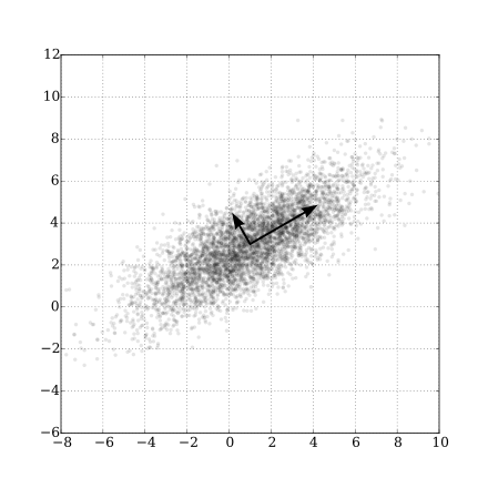
PCA determines othogonal components in \(\mathbb{R}^d\) using the SVD decomposition of the covariance matrix, and determines d eigenvector / eigenvalue pairs, known as “principal components”. Each eigenvector defines an orthogonal axis in \(\mathbb{R}^d\) that aligns along maximal variance. The variance oriented alignment is easy to see in the decomposition of a 2-dimensional data set depicted below (source: Wikipedia):

Dimensional reduction is achieved by selecting the k < d eigenvectors with the highest magnitude (variance). The original data can be reconstructed (with some error) from the k eignvectors with a linear combination.
Problems with PCA
However, PCA is rarely going to be an effective approach for dimensional reduction in machine learning data sets. There are two fundamental problems with PCA used in this context:
- PCA has no conditioning on outcome
- should be performed, in some way, on conditonal distribution \(p(x \vert f(x))\)
- The variance of features may have little to do with \(p(f(x) \vert x)\)
- the transfer function y = f(x) may be non-linear or scaled in such a way that the covariance of x is not representative.
Consider the above figure showing the principal component decomposition of a 2 dimensional feature set. If we use PCA to reduce from 2 dimensions to 1 dimension, the eigenvector with the largest eigenvalue (the magnitude) would be chosen. In this case the vector aligned at ~30 degrees would be the selected vector.
However, this vector may not be aligned in importance with the underlying function f(x). In dimensional reduction we want to select components that align with the largest transfer function (f(x)) sensitivities. These will correspond to the partial derivatives of f(x) with respect to each feature (and not necessarily the variance of features).
By way of example, supposing we want to use ML to learn the following function:
\[f(\vec{x}) = \begin{bmatrix} 100 & 0 \\ 0 & 1 \end{bmatrix} \begin{bmatrix} cos (-\pi/6) & -sin (-\pi/6) \\ sin (-\pi/6) & cos (-\pi/6) \end{bmatrix} \vec{x} + \vec{\epsilon}\]The above function has 100x the sensitivity to the 2nd PCA component in the features and very little sensitivity to the 1st PCA component. In selecting the 1st component (the component with highest variance), PCA has selected a noisy variable with little impact on f(x). Training a model for f(x) on the PCA reduced feature set would produce a very low accuracy, given that most of the information was in the 2nd component.
While the above example was contrived, in practice I find that PCA often emphasizes the wrong features when performing dimensional reduction for my data sets.
LDA
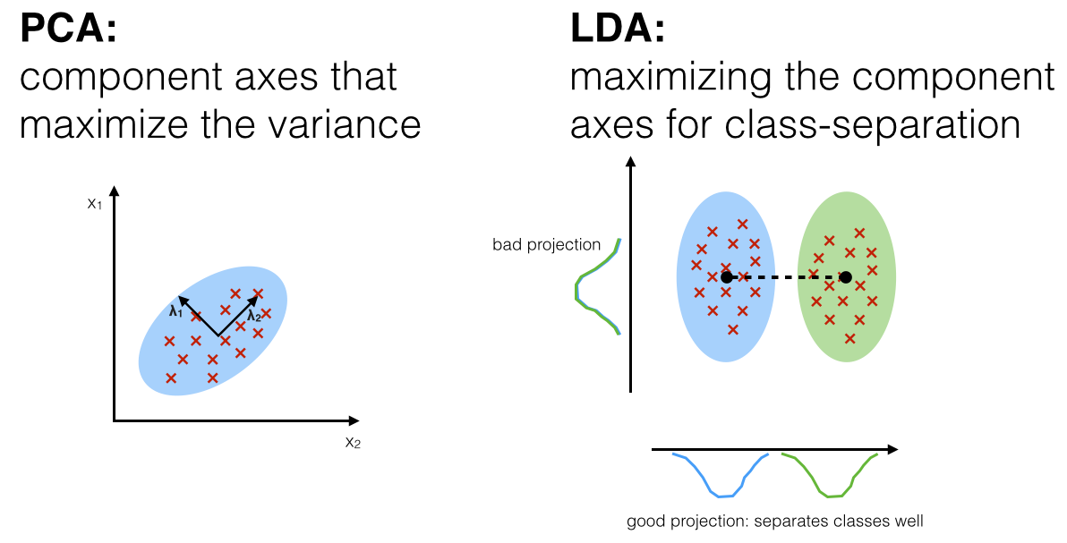
LDA solves some of the problems of PCA, where instead of determining orthogonal components on maximum variance axes, determines components than maximize linear class-separation. Sebastian Raschka has written an excellent article on Linear Discriminant Analysis, contrasting to PCA . Borrowing a diagram from his blog:
 (source: Sebastian Raschka's blog)
Deficiencies of LDA
LDA will often perform better than PCA due to the explicit selection of components that maximize class separation. There are, however, some issues that may make it unsuitable for a given data set:
- less effective for non-linear relationships
- if the classes / features are not linearly separable, requiring non-linear separation, this approach will fail
- use of centroids to define barycenter for each feature distribution
- this is appropriate for relatively symmetric distributions, but would tend to be unrepresentative for many other distributions present in financial data.
Auto-Encoders
Auto-Encoders present a very interesting approach to dimensional reduction. The approach involves creating a deep neural network with:
- d inputs (for feature dimension \(\mathbb{R}^d\))
- hidden layers to effect the encoding and decoding
- an internal layer with k nodes between the encoder and decoder (to obtain k-dimensional features)
- an output layer with d nodes (to reconstitute the d-dimensional input features)
The idea is that we want to train the encoder to generate features in \(\mathbb{R}^k\) space, with fidelity to reproduce the d-dimensional features from the k-dimensional reduced feature set.

The network is trained on the same input and outputs, such that the hidden internal k-dimensional layer learns the optimal representation in \(\mathbb{R}^k\) sufficient to reproduce \(\mathbb{R}^d\) with minimal error.
While deep-learning ANNs allow for non-linearities (unlike PCA), auto-encoders also suffer from inability to classify the relative importance of features based on feature -> class fidelity.
Intermediate Conclusions
Each approach has drawbacks and may or may not be suitable for a given data set:
- PCA has significant drawbacks (probably the least effective of the 3):
- negative: cannot select based on discrimination between classes (or outcome)
- negative: linear transformation
- LDA improves on PCA:
- positive: determines components that maximize discrimination between classes
- negative: requires linear separability
- negative: use of centroids will fail with non-symmetric distributions
- Auto-Encoders:
- positive: can embody non-linearities in the transformation of features
- positive: allow for higher compression of dimension than PCA for certain data sets
- negative: cannot select based on discrimination between classes (or outcome)
Ideally we want a dimensional reduction technique that:
- is aware of the relationship between features and outcome
- choosing features that maximize resolution of p(f(x) = y | x)
- can deal with a wide variety of feature distributions
- for example distributions with fat tails, exponential, etc
- non-linear
Next
In the next post will describe a distribution based approach and compare to a ML model importance based approach.