Pricing Deribit Options
We have been working on some option strategies and wanted to get a sense of how well BTC and ETH options are priced on Deribit, i.e. is there a substantial IV premium over realized volatility or are options fairly priced. At first glance, based on the documentation, it seemed that Deribit options were Europeans on spot or spot equivalent. On closer inspection, however, and with some follow-ups with deribit, determined that this is actually a much more complex product (to price).
It turns out that the options have the following features:
- are “asian” options, where the payout is based on the average of the underlier over some observation window
- in particular these options use the average price over a 30 min or 5 min window in determining the price at expiry
- the average is an artithmetic average as opposed to a geometric average. Asian option pricing for arithmetic averages is more complicated as does not allow a closed-form solution.
- variable averaging window depending on whether the expiry is matched 1:1 with a future
- a 30 minute window is used for options where the expiry does not align exactly with a future
- a 5 minute window is used for options where the expiry aligns with a future
- The underlier is a future or synthetic future, as opposed to spot
- in practice, the future should converge to spot by expiry, but may have some different dynamics in between
Our original goal was to back out the Black-Scholes equivalent implied volatilities (IV) and determine the volatility surface. It is worth noting that Black Scholes (BS) has well known drawbacks (model error) in related to its assumptions:
- constant volatility across the lifetime of the option
- constant interest rate across the lifetime of the option
- log normal price distribution (under estimates the tails)
In order to back out the BS IV for deribit options we will need to:
- work out how to price each “asian” option, given:
- time to expiry, price of underlier, assumed risk-free-rate, volatility
- interatively adjust volatility to determine an implied volatility that reprices to the premium
- i.e. f(spot price, time, rfr, iv) = observed premium
Pricing an Asian Option
We cannot use the Black-Schole formula for European options to price an Asian Option, however we can borrow the the price process assumed in BS. The Black-Scholes formulation of the price process evolves according to the following SDE:
\[\partial{S_t} = rS_t\partial{t} + \sigma S_t \partial{W_t}\]where \(S_t\) is the price, \(r\) is the risk-free-rate, \(\sigma\) the volatility, \(W_t\) is a Weiner process. We will use this later in our solution for pricing an Asian option.
The averaging period of an Asian option is path dependent: i.e. we care about where the price went across the averaging period as opposed to the terminal price at expiry. Due to this path dependency, while there are some closed form approximations, the most accurate way to evaluate these options is with a Monte Carlo (MC) technique.
With the MC technique, we simulate many price paths to option expiry using the above Black-Scholes SDE. We observe the price at K points within the averaging period to determine the terminal price to be used for the option value at expiry.
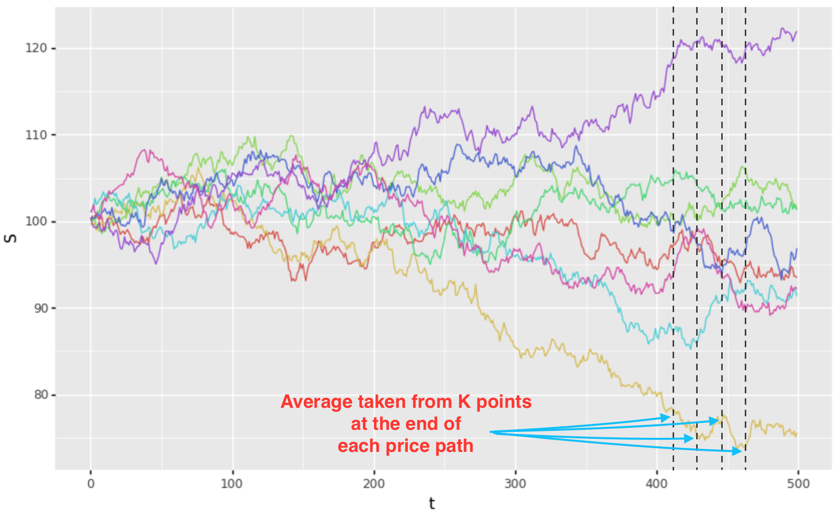
Given, say, 100K paths, for each path \(i\) we compute the average \(A_i\) during the observation period and evaluate the payoff of for a call option to be:
\[e^{-r t} \, max(A_i - K, 0)\]where \(K\) is the strike, \(r\) is the risk free rate, and \(A_i\) is the observed average on that path. We can determine the premium to be the expected value of the option payoff, or in other words, the average payoff of all of the paths.
\[premium = \frac{1}{n} \sum_{i = 1}^n e^{-r t} \, payoff \, (path_i)\]Implementation
The first thing to note is that we need a discretized form of the BS price process. Integrating for some \(\Delta t\), this works out to be:
\[S_{t+\Delta t} = S_t e^{(r - \tfrac{1}{2} \sigma^2)\Delta t + \sigma \sqrt{\Delta t}W_t}\]Using the above we can use this to evolve a path for K time steps until expiry, expressing \(S_{t+\Delta t}\) in terms of the prior price \(S_t\) recursively.
We would like to limit the amount of computation required to evaluate a path. Noting that prior to the averaging period, we have no price path dependency, we can avoid computing the path from \(t = 0\) until \(T - 30min\). This can be accomplished by:
- sampling the “prior path” up to \(S_{T - 30m}\) from the BS forward price distribution
- given by the above discretization, where \(\Delta t = T - 30m\)
- using the sampled price \(S_{T - 30m}\), create a path with 30 additional prices
- each price on the path post T - 30min will be used in the average for that particular path
- we assume here, that the average is composed of 1min samples
There are other tricks we can deploy to reduce the computation time or improve accuracy, for example:
- choose an appropriate random number generator which has a distribution suitable for MC
- Sobol and Halton sequences are excellent for MC
- precompute the random normal samples and reuse in each calculation
- the cost of generating random numbers on the fly can be substantial
- antithetic variate
- for every random draw can apply the + and - variation, creating 2 paths for every 1.
- variance reduction
- reframe the variable (if possible) such that evaluating a problem with reduced variance, requiring fewer paths
Code
Here is a snippet of code for the simple case where we are pricing an asian option before the averaging period has started:
- let W[t] be a precomputed cache of random normals drawn from a Sobol sequence
- let t = time until maturity (in 1 / 365.25 units)
- let spot = the underlier at the time of evaluation (the future price in this case)
- let r = risk-free-rate (interest rate)
- let dir = 1 = call, -1 = put
- let sigma = volatility
val T1min = 1.0 / (365.25 * 24 * 60.0)
val sqrtT1m = sqrt(T1min)

val Tprior = t - averageperiod * T1min
val sqrtTp = sqrt(Tprior)

var cpayoff = 0.0
for (pathi in 0 until paths / 2) {
    val ri = pathi * (averageperiod+1)

    // compute 2 antithetic paths up to average measurement period: T - observation window
    var path1 = spot * exp((r - 0.5 * sigma * sigma) * Tprior + sigma * sqrtTp * W[ri])
    var path2 = spot * exp((r - 0.5 * sigma * sigma) * Tprior - sigma * sqrtTp * W[ri])

    // compute average period for the 2 antithetic paths
    var cmean1 = 0.0
    var cmean2 = 0.0
    for (i in 1 .. averageperiod) {
        path1 = path1 * exp((r - 0.5 * sigma * sigma) * T1min + sigma * sqrtT1m * W[ri+i])
        path2 = path2 * exp((r - 0.5 * sigma * sigma) * T1min - sigma * sqrtT1m * W[ri+i])

        cmean1 += path1
        cmean2 += path2
    }

    // compute payoffs
    val mean1 = cmean1 / averageperiod
    val mean2 = cmean2 / averageperiod

    cpayoff += max (dir * (mean1 - strike), 0.0)
    cpayoff += max (dir * (mean2 - strike), 0.0)
}

val df = Math.exp(-r * t)
val premium = df * cpayoff / paths
If the we are already in the averaging period then the code would be adjusted to combine the “fixings” (historical price points) and the remaining path projected with MC.
Calculating IV
Given the ability to, now, price an asian option, we can backout the value of sigma (\(\sigma\)), our implied volatilty. Making use of zbrent, or another efficient root finder, can solve for:
\[pv(spot, time, rfr, sigma) - premium = 0\]for some range of sigma.
Notes
- deribit actually uses 6 second sampling rather than a 1min sampling during the average window
- my current Deribit data is at 1min granularity, so assuming a different sampling frequency.
- deribit does selectively use either 30min or 5min windows for the average as described above.
- deribit’s published IVs are priced assuming that the option is a European Black-Scholes
- their IV is not correct, so use at your own risk
- the option underlier may be a blend of the two straddling futures if there is no matching future